🧑💻복습/파이썬
파이썬 AI 프로젝트 적용 XOR 문제 해결과 주요 머신러닝 알고리즘 소개: SVM, Linear 모델, Tree 모델, Ensemble 모델, KFold, Feature Importances
우동한그릇
2023. 5. 15. 20:52
반응형

1. XOR 문제의 해결
import numpy as np
from sklearn.linear_model import Perceptron
from sklearn.svm import SVC, SVR, LinearSVC, LinearSVR
from sklearn.metrics import accuracy_score
from keras.models import Sequential
from keras.layers import Dense

#1. 데이터
# MLP모델 구성하여 ACC=1.0 만들기
x_data = [[0,0], [0,1], [1,0], [1,1]]
y_data = [0, 1, 1, 0]

#2. 모델
model = Sequential()
model.add(Dense(32, input_dim=2))
model.add(Dense(64, activation = 'relu'))
model.add(Dense(64, activation = 'relu'))
model.add(Dense(64, activation = 'relu'))
model.add(Dense(1, activation='sigmoid'))
 # sklearn의 perceptron과 동일

#3. 컴파일, 훈련
model.compile(loss='binary_crossentropy',
              optimizer='adam',
              metrics='acc')

model.fit(x_data, y_data, batch_size=1, epochs=100)


#4. 평가, 예측
loss,acc = model.evaluate(x_data, y_data)
y_predict = model.predict(x_data)

print(x_data, "의 결과 : ", y_predict)
print('모델의 loss : ', loss)
print('acc : ', acc)

# MLP모델 구성하여 ACC=1.0 만들기
# 모델의 loss :  0.00042129121720790863
# acc :  1.0
2. SVM 모델 (SVC, SVR)
import numpy as np
from sklearn.linear_model import Perceptron
from sklearn.svm import SVC, SVR, LinearSVC, LinearSVR
from sklearn.metrics import accuracy_score

#1. 데이터

x_data = [[0,0], [0,1], [1,0], [1,1]]
y_data = [0, 1, 1, 0]


#2. 모델
model = SVC() #MLP (multi layer perceptron)

#3. 훈련
model.fit(x_data, y_data)

#4. 평가, 예측
result = model.score(x_data, y_data)
print('모델 score : ', result)

y_predict = model.predict(x_data)
print(x_data, "의 결과 : ", y_predict)

acc = accuracy_score(y_data, y_predict)
print('acc : ', acc)

# SVC 퍼셉트론
# 모델 score :  1.0
# [[0, 0], [0, 1], [1, 0], [1, 1]] 의 결과 :  [0 1 1 0]
# acc :  1.0
3. Linear 모델
(Perceptron, LogisticRegression은 분류모델, LinearRegression 회귀모델)
[SVR 회귀모델]
#1. 실습 svm 모델과 나의 tf keras 모델 성능 비교하기
#1. iris
#2. cancer
#3. wine
#4. cailimport numpy as np
import numpy as np
from sklearn.linear_model import Perceptron
from sklearn.svm import SVR, LinearSVR
from sklearn.metrics import accuracy_score
from keras.models import Sequential
from keras.layers import Dense
from sklearn.datasets import load_breast_cancer
from sklearn.datasets import load_wine
from sklearn.model_selection import train_test_split
from sklearn.datasets import fetch_california_housing
import tensorflow as tf
tf. random.set_seed(100) # weigth에 난수값 조절

#1. 데이터
datasets = fetch_california_housing()
x = datasets['data']
y = datasets['target']

print(x.shape, y.shape) # (150, 4) (150,)
print('y의 라벨값 : ', np.unique(y))    # y의 라벨값 :  [0 1 2]

#2. 모델
model = SVR()

#3. 훈련
model.fit(x,y)

#4. 평가, 예측
result = model.score(x, y)
print('결과 cail SVR acc : ', result)


#
#2. 모델
model = LinearSVR()

#3. 훈련
model.fit(x,y)

#4. 평가, 예측
result = model.score(x, y)
print('결과 cail LinearSVR acc : ', result)


####

#2. 모델
model = SVR()
x_train, x_test, y_train, y_test = train_test_split(

    x,y,train_size=0.7, random_state=100, shuffle= True
)

#3. 훈련
model.fit(x_train,y_train)

#4. 평가, 예측
result = model.score(x_test, y_test)
print('결과 svr mlp acc : ', result)


# 결과 cail SVR acc :  -0.01658668690926901
# 결과 cail LinearSVR acc :  -0.41929123956268755
# 결과 svr mlp acc :  -0.01663695941103427
[SVC 분류모델]
#1. 실습 svm 모델과 나의 tf keras 모델 성능 비교하기
#1. iris
#2. cancer
#3. wine
#4. cailimport numpy as np
import numpy as np
from sklearn.linear_model import Perceptron
from sklearn.svm import SVC, LinearSVC
from sklearn.metrics import accuracy_score
from keras.models import Sequential
from keras.layers import Dense
from sklearn.datasets import load_breast_cancer
from sklearn.model_selection import train_test_split
from sklearn.datasets import fetch_california_housing

#1. 데이터
datasets = load_breast_cancer()
x = datasets['data']
y = datasets['target']

print(x.shape, y.shape) # (150, 4) (150,)
print('y의 라벨값 : ', np.unique(y))    # y의 라벨값 :  [0 1 2]

#2. 모델
model = SVC()

#3. 훈련
model.fit(x,y)

#4. 평가, 예측
result = model.score(x, y)
print('결과 cance svc acc : ', result)

# ####
#2. 모델
model = LinearSVC()

#3. 훈련
model.fit(x,y)

#4. 평가, 예측
result = model.score(x, y)
print('결과 cancer LinearSVC acc : ', result)


#2. 모델
model = SVC()
x_train, x_test, y_train, y_test = train_test_split(

    x,y,train_size=0.7, random_state=100, shuffle= True
)

#3. 훈련
model.fit(x_train,y_train)

#4. 평가, 예측
result = model.score(x_test, y_test)
print('결과 cancer mlp acc : ', result)


#결과 cance svc acc :  0.9226713532513181
# 결과 cancer LinearSVC acc :  0.9244288224956063
# 결과 cancer mlp acc :  0.9064327485380117
4. Tree 모델 (DecisionTreeClassifier, DecisionTreeRegressor)
[DecisionTreeRegressor]
import numpy as np
from keras.models import Sequential
from keras.layers import Dense, Dropout
from sklearn.model_selection import train_test_split
from sklearn.metrics import r2_score
from sklearn.datasets import fetch_california_housing
# from sklearn.datasets import load_boston #윤리적 문제로 제공안됨
from sklearn.svm import SVR, LinearSVR
from sklearn.preprocessing import MinMaxScaler, StandardScaler
from sklearn.preprocessing import MaxAbsScaler, RobustScaler
from sklearn.tree import DecisionTreeRegressor

#1. 데이터
# datasets = load_boston()
datasets = fetch_california_housing()

x = datasets.data
# ['MedInc', 'HouseAge', 'AveRooms', 'AveBedrms', 'Population', 'AveOccup', 'Latitude', 'Longitude']
y = datasets.target
# MedInc 블록 그룹의 중간 소득
# HouseAge 중간 블록 그룹의 주택 연령
# AveRooms 가구당 평균 객실 수
# AveBedrms 가구당 평균 침실 수
# Population 인구 블록 그룹 인구
# AveOccup 평균 가구 구성원 수
# Latitude 위도 블록 그룹 위도
# Longitude 경도 블록 그룹 경도

print(datasets.feature_names)
print(datasets.DESCR)

print(x.shape) #(20640, 8)
print(y.shape) #(20640,)

model = DecisionTreeRegressor
x_train, x_test, y_train, y_test = train_test_split(
    x, y, train_size=0.7, random_state=100, shuffle=True
)

# scaler 적용
# scaler = MinMaxScaler()
scaler = StandardScaler()
# scaler = MaxAbsScaler()
#scaler = RobustScaler()

scaler.fit(x_train)
x_train = scaler.fit_transform(x_train)
x_test = scaler.transform(x_test)


#2. 모델구성
model = Sequential()
model.add(Dense(8, input_dim=8)) # print(x_train.shape) # (14447, 8) 열 숫자
model.add(Dense(100))
model.add(Dropout(0.25))
model.add(Dense(100))
model.add(Dropout(0.25))
model.add(Dense(100))
model.add(Dense(100))
model.add(Dense(1)) # 회귀분석이므로 출력층은 1

#3. 컴파일, 훈련
model.compile(loss='mse', optimizer='adam')
model.fit(x_train, y_train, epochs=500, batch_size=125) #epochs 반복횟수

#4. 평가, 예측
loss = model.evaluate(x_test, y_test)
print('loss : ', loss)

y_predict = model.predict(x_test)

r2 = r2_score(y_test, y_predict)
print('r2스코어 : ', r2)

#loss :  0.506873607635498
#r2스코어 :  0.617474494949859


# loss :  0.3207322657108307
# acc :  0.9259259104728699
[DecisionTreeClassifier]
import numpy as np
from keras.models import Sequential
from keras.layers import Dense
from sklearn.model_selection import train_test_split
from sklearn.metrics import r2_score, accuracy_score
from sklearn.datasets import load_iris
from sklearn.preprocessing import MinMaxScaler, StandardScaler
from sklearn.preprocessing import MaxAbsScaler, RobustScaler
import time
from sklearn.svm import SVC, LinearSVC
from sklearn.tree import DecisionTreeClassifier

#1. 데이터
datasets = load_iris()
print(datasets.DESCR)
print(datasets.feature_names)
#['sepal length (cm)', 'sepal width (cm)', 'petal length (cm)', 'petal width (cm)']

x = datasets.data
y = datasets.target
print(x.shape,y.shape) # (150, 4) (150,) #input_dim = 4

model = DecisionTreeClassifier()
x_train, x_test, y_train, y_test = train_test_split(
    x, y, train_size=0.7, random_state=100, shuffle=True
)

print(x_train.shape, y_train.shape)
print(x_test.shape, y_test.shape)
print(y_test)

# scaler 적용
# scaler = MinMaxScaler()
scaler = StandardScaler()
# scaler = MaxAbsScaler()
#scaler = RobustScaler()

scaler.fit(x_train)
x_train = scaler.fit_transform(x_train)
x_test = scaler.transform(x_test)

#2. 모델 구성
model = Sequential()
model.add(Dense(100,input_dim=4))
model.add(Dense(100))
model.add(Dense(100))
model.add(Dense(500))
model.add(Dense(3, activation='softmax'))

#3.컴파일, 훈련
model.compile(loss='sparse_categorical_crossentropy', optimizer='adam',
              metrics=['accuracy'])

start_time = time.time()
model.fit(x_train, y_train, epochs=100, batch_size=100)
end_time = time.time() - start_time

#4. 평가,예측
# y_predict = model.predict(x_test)
# y_predict = np.round(y_predict)

# loss= model.evaluate(x_test, y_test)
# acc = accuracy_score(y_test, y_predict)
#
y_predict = model.predict(x_test)
y_predict = np.argmax(y_predict, axis=1)
#

print(y_predict)
loss= model.evaluate(x_test, y_test)
acc = accuracy_score(y_test, y_predict)

# np.argmax(,axis=n) 함수는 배열에서 가장 큰 값의
# 인덱스를 반환하는 함수입니다.
# axis=1을 지정하여 각 행에서 가장 큰 값의 인덱스를 추출하면,
# 다중 클래스로 예측된 결과를 얻을 수 있습니다.
# axis = 0 (행), axis = 1 (열)

print('loss : ', loss)
print('acc : ', acc)
print('걸린시간 : ', end_time)


# loss :  [0.11477744579315186, 0.9555555582046509]
# acc :  0.9555555555555556
# 걸린시간 :  0.9926300048828125

# sclaer 적용
# loss :  [0.049853190779685974, 0.9777777791023254]
# acc :  0.9777777777777777
# 걸린시간 :  0.9749109745025635
5. Ensemble 모델 (RandomForestClassifier, RandomForestRegressor)
[DecisionTreeClassifier]
import numpy as np
from sklearn.datasets import load_iris
from sklearn.model_selection import train_test_split, KFold, StratifiedKFold
from sklearn.model_selection import cross_val_score, cross_validate, cross_val_predict
from sklearn.preprocessing import MinMaxScaler
from sklearn.utils import all_estimators
from sklearn.metrics import r2_score, accuracy_score
from sklearn.ensemble import RandomForestRegressor, RandomForestClassifier


import warnings
warnings.filterwarnings('ignore')

#1.데이터
datasets = load_iris()
x = datasets.data
y = datasets.target

x_train, x_test, y_train, y_test = train_test_split(
    x, y, train_size=0.8, shuffle=True, random_state=42 # valdiation data포함
)

#kfold
n_splits = 5
random_state=42
kfold = StratifiedKFold(n_splits=n_splits,
                             shuffle=True,
                             random_state=random_state)

scaler = MinMaxScaler()
scaler.fit(x_train)
x = scaler.transform(x)
x_train = scaler.fit_transform(x_train)
x_test = scaler.transform(x_test)
# x_test = scaler.transform(x_test)

#2. 모델
model = RandomForestClassifier()

#3.훈련
model.fit(x_train, y_train)

#4. 결과
score = cross_val_score(model,
                        x_train, y_train,
                        cv=kfold)   #   crossvalidation

print(score)
y_predict = cross_val_predict(model,
                              x_test, y_test,
                              cv=kfold)
y_predict = np.round(y_predict).astype(int)
# print('cv predict : ', y_predict)
acc = accuracy_score(y_test, y_predict)
print('cv RandomForestClassifier iris pred acc : ', acc)
#[0.91666667 0.95833333 0.91666667 0.83333333 1.        ]
# cv RandomForestClassifier iris pred acc :  0.9666666666666667


# [0.95833333 0.95833333 0.875      0.95833333 0.91666667]
# cv RandomForestClassifier iris pred acc :  0.9666666666666667
[RandomForestRegressor]
import numpy as np
from sklearn.datasets import fetch_california_housing
from sklearn.model_selection import train_test_split, KFold, StratifiedKFold
from sklearn.model_selection import cross_val_score, cross_validate, cross_val_predict
from sklearn.preprocessing import MinMaxScaler
from sklearn.utils import all_estimators
from sklearn.metrics import r2_score, accuracy_score
from sklearn.ensemble import RandomForestRegressor, RandomForestClassifier


import warnings
warnings.filterwarnings('ignore')

#1.데이터
datasets = fetch_california_housing()
x = datasets.data
y = datasets.target

x_train, x_test, y_train, y_test = train_test_split(
    x, y, train_size=0.8, shuffle=True, random_state=42 # valdiation data포함
)

#kfold
n_splits = 5
random_state=42
kfold = KFold(n_splits=n_splits,
                             shuffle=True,
                             random_state=random_state)

scaler = MinMaxScaler()
scaler.fit(x_train)
x = scaler.transform(x)
x_train = scaler.fit_transform(x_train)
x_test = scaler.transform(x_test)
# x_test = scaler.transform(x_test)

#2. 모델
model = RandomForestRegressor()

#3.훈련
model.fit(x_train, y_train)

#4. 결과
score = cross_val_score(model,
                        x_train, y_train,
                        cv=kfold)   #   crossvalidation

print(score)
y_predict = cross_val_predict(model,
                              x_test, y_test,
                              cv=kfold)
#y_predict = np.round(y_predict).astype(int)
# print('cv predict : ', y_predict)
r2 = r2_score(y_test, y_predict)
print('cv RandomForestClassifier iris pred acc : ', r2)
#[0.91666667 0.95833333 0.91666667 0.83333333 1.        ]
# cv RandomForestClassifier iris pred acc :  0.9666666666666667


# [0.95833333 0.95833333 0.875      0.95833333 0.91666667]
# cv RandomForestClassifier iris pred acc :  0.9666666666666667


####feature importaces

print(model, ":", model.feature_importances_)

import matplotlib.pyplot as plt
n_features = datasets.data.shape[1]
plt.barh(range(n_features), model.feature_importances_,align='center')
plt.yticks(np.arange(n_features), datasets.feature_names)
plt.title('cali Feature Importances')
plt.ylabel('Feature')
plt.xlabel('importances')
plt.ylim(-1, n_features) # 가로출력

plt.show()
6. All_Estimator (알고리즘 출력하면서 정확도 찾기)
import numpy as np
from sklearn.datasets import load_breast_cancer
from sklearn.model_selection import train_test_split
from sklearn.preprocessing import MinMaxScaler
from sklearn.utils import all_estimators
from sklearn.metrics import r2_score, accuracy_score

import warnings
warnings.filterwarnings('ignore')

#1.데이터
datasets = load_breast_cancer()
x = datasets.data
y = datasets.target

x_train, x_test, y_train, y_test = train_test_split(
    x, y, train_size=0.7, random_state=42, shuffle=True
)

scaler = MinMaxScaler()
x_train = scaler.fit_transform(x_train)
x_test = scaler.transform(x_test)

#2. 모델
allAlgorithms = all_estimators(type_filter='classifier')
print('allAlgorithms : ', allAlgorithms)
print('total : ', len(allAlgorithms)) # 41개

#3. 출력
for (name, algorithm) in allAlgorithms :
    try :
        model = algorithm()
        model.fit(x_train, y_train)
        y_predict = model.predict(x_test)
        acc = accuracy_score(y_test, y_predict)
        print(name, '의 정답률 : ', acc)
    except :
        print(name, '안나온 놈 !')
7. KFold 와 StratifiedKFold (회귀분석과 분류모델)
[KFold]
import numpy as np
from sklearn.datasets import load_wine
from sklearn.model_selection import train_test_split, KFold
from sklearn.model_selection import cross_val_score, cross_validate, cross_val_predict
from sklearn.preprocessing import MinMaxScaler
from sklearn.utils import all_estimators
from sklearn.metrics import r2_score, accuracy_score
from sklearn.ensemble import RandomForestRegressor, RandomForestClassifier


import warnings
warnings.filterwarnings('ignore')

#1.데이터
datasets = load_wine()
x = datasets.data
y = datasets.target

x_train, x_test, y_train, y_test = train_test_split(
    x, y, train_size=0.8, shuffle=True, random_state=42 # valdiation data포함
)

#kfold
n_splits = 5
random_state=42
kfold = KFold(n_splits=n_splits, shuffle=True, random_state=random_state)

scaler = MinMaxScaler()
scaler.fit(x_train)
x = scaler.transform(x)
x_train = scaler.fit_transform(x_train)
x_test = scaler.transform(x_test)
# x_test = scaler.transform(x_test)

#2. 모델
model = RandomForestRegressor()

#3.훈련
model.fit(x_train, y_train)

#4. 결과
score = cross_val_score(model,
                        x_train, y_train,
                        cv=kfold)   #   crossvalidation

print(score)
y_predict = cross_val_predict(model,
                              x_test, y_test,
                              cv=kfold)
y_predict = np.round(y_predict).astype(int)
# print('cv predict : ', y_predict)
r2 = r2_score(y_test, y_predict)
#acc = accuracy_score(y_test, y_predict)
print('cv RandomForestClassifie cali pred acc : ', r2)

#[0.92044174 0.93128764 0.86083611 0.94454865 0.9748    ]
# cv RandomForestClassifie cali pred acc :  0.7619047619047619
[StratifiedKFold]
import numpy as np
from sklearn.datasets import load_iris
from sklearn.model_selection import train_test_split, KFold, StratifiedKFold
from sklearn.model_selection import cross_val_score, cross_validate, cross_val_predict
from sklearn.preprocessing import MinMaxScaler
from sklearn.utils import all_estimators
from sklearn.metrics import r2_score, accuracy_score
from sklearn.ensemble import RandomForestRegressor, RandomForestClassifier


import warnings
warnings.filterwarnings('ignore')

#1.데이터
datasets = load_iris()
x = datasets.data
y = datasets.target

x_train, x_test, y_train, y_test = train_test_split(
    x, y, train_size=0.8, shuffle=True, random_state=42 # valdiation data포함
)

#kfold
n_splits = 5
random_state=42
kfold = StratifiedKFold(n_splits=n_splits,
                             shuffle=True,
                             random_state=random_state)

scaler = MinMaxScaler()
scaler.fit(x_train)
x = scaler.transform(x)
x_train = scaler.fit_transform(x_train)
x_test = scaler.transform(x_test)
# x_test = scaler.transform(x_test)

#2. 모델
model = RandomForestClassifier()

#3.훈련
model.fit(x_train, y_train)

#4. 결과
score = cross_val_score(model,
                        x_train, y_train,
                        cv=kfold)   #   crossvalidation

print(score)
y_predict = cross_val_predict(model,
                              x_test, y_test,
                              cv=kfold)
y_predict = np.round(y_predict).astype(int)
# print('cv predict : ', y_predict)
acc = accuracy_score(y_test, y_predict)
print('cv RandomForestClassifier iris pred acc : ', acc)
#[0.91666667 0.95833333 0.91666667 0.83333333 1.        ]
# cv RandomForestClassifier iris pred acc :  0.9666666666666667


# [0.95833333 0.95833333 0.875      0.95833333 0.91666667]
# cv RandomForestClassifier iris pred acc :  0.9666666666666667
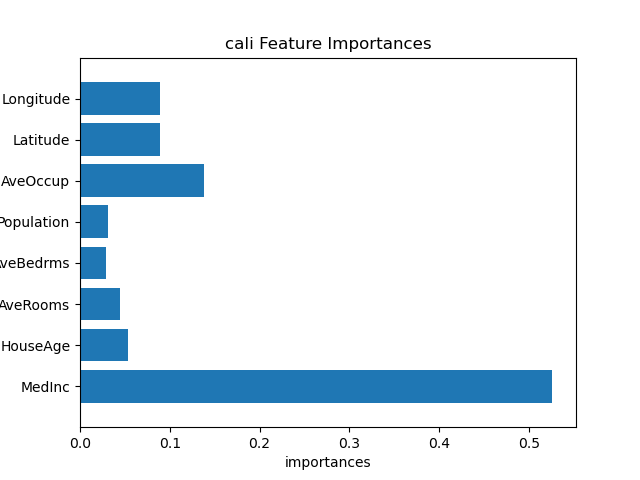
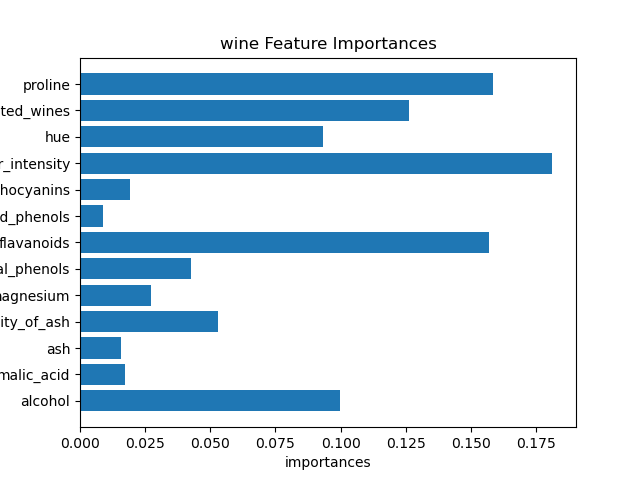
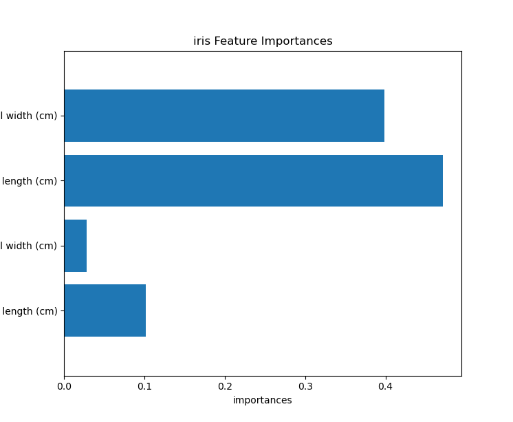
8. Feature Importances (피쳐 중요도)
import numpy as np
from sklearn.datasets import fetch_california_housing
from sklearn.model_selection import train_test_split, KFold, StratifiedKFold
from sklearn.model_selection import cross_val_score, cross_validate, cross_val_predict
from sklearn.preprocessing import MinMaxScaler
from sklearn.utils import all_estimators
from sklearn.metrics import r2_score, accuracy_score
from sklearn.ensemble import RandomForestRegressor, RandomForestClassifier


import warnings
warnings.filterwarnings('ignore')

#1.데이터
datasets = fetch_california_housing()
x = datasets.data
y = datasets.target

x_train, x_test, y_train, y_test = train_test_split(
    x, y, train_size=0.8, shuffle=True, random_state=42 # valdiation data포함
)

#kfold
n_splits = 5
random_state=42
kfold = KFold(n_splits=n_splits,
                             shuffle=True,
                             random_state=random_state)

scaler = MinMaxScaler()
scaler.fit(x_train)
x = scaler.transform(x)
x_train = scaler.fit_transform(x_train)
x_test = scaler.transform(x_test)
# x_test = scaler.transform(x_test)

#2. 모델
model = RandomForestRegressor()

#3.훈련
model.fit(x_train, y_train)

#4. 결과
score = cross_val_score(model,
                        x_train, y_train,
                        cv=kfold)   #   crossvalidation

print(score)
y_predict = cross_val_predict(model,
                              x_test, y_test,
                              cv=kfold)
#y_predict = np.round(y_predict).astype(int)
# print('cv predict : ', y_predict)
r2 = r2_score(y_test, y_predict)
print('cv RandomForestClassifier iris pred acc : ', r2)
#[0.91666667 0.95833333 0.91666667 0.83333333 1.        ]
# cv RandomForestClassifier iris pred acc :  0.9666666666666667


# [0.95833333 0.95833333 0.875      0.95833333 0.91666667]
# cv RandomForestClassifier iris pred acc :  0.9666666666666667


####feature importaces

print(model, ":", model.feature_importances_)

import matplotlib.pyplot as plt
n_features = datasets.data.shape[1]
plt.barh(range(n_features), model.feature_importances_,align='center')
plt.yticks(np.arange(n_features), datasets.feature_names)
plt.title('cali Feature Importances')
plt.ylabel('Feature')
plt.xlabel('importances')
plt.ylim(-1, n_features) # 가로출력

plt.show()
실습
각 boost 계열 모델 (iris, cancer, wine, california)
팀 프로젝트에 1번, 2번 적용
[Lightgbmboost]
pip install xgboost

pip install catboost

pip install lightgbm

import numpy as np
import pandas as pd
from keras.models import Sequential
from keras.layers import Dense, Dropout
from sklearn.model_selection import train_test_split
from sklearn.metrics import r2_score

import numpy as np
from sklearn.datasets import fetch_california_housing
from sklearn.model_selection import train_test_split, KFold, StratifiedKFold
from sklearn.model_selection import cross_val_score, cross_validate, cross_val_predict
from sklearn.preprocessing import MinMaxScaler
from sklearn.utils import all_estimators
from sklearn.metrics import r2_score, accuracy_score
from sklearn.ensemble import RandomForestRegressor, RandomForestClassifier


import warnings
warnings.filterwarnings('ignore')

#1. 데이터
path = './'
datasets = pd.read_csv(path + 'train.csv')

print(datasets.columns)
#print(datasets.head(7))

# 1. x,y Data
x = datasets[['6~7_ride', '7~8_ride', '8~9_ride',
       '9~10_ride', '10~11_ride', '11~12_ride', '6~7_takeoff', '7~8_takeoff',
       '8~9_takeoff', '9~10_takeoff', '10~11_takeoff', '11~12_takeoff']]
y = datasets[['18~20_ride']]

x = x.astype('int64')

print(x.info())

x_train, x_test, y_train, y_test = train_test_split(
    x, y, train_size=0.8, shuffle=True, random_state=42 # valdiation data포함
)

#kfold
n_splits = 5
random_state=77
kfold = KFold(n_splits=n_splits,
                             shuffle=True,
                             random_state=random_state)

scaler = MinMaxScaler()
scaler.fit(x_train)
x = scaler.transform(x)
x_train = scaler.fit_transform(x_train)
x_test = scaler.transform(x_test)

from lightgbm import LGBMRegressor
model = LGBMRegressor()

#3.훈련
model.fit(x_train, y_train)

#4. 결과
score = cross_val_score(model,
                        x_train, y_train,
                        cv=kfold)   #   crossvalidation

print(score)
y_predict = cross_val_predict(model,
                              x_test, y_test,
                              cv=kfold)

r2 = r2_score(y_test, y_predict)
print('lightgbm r2 : ', r2)

import matplotlib.pyplot as plt

n_features = x.shape[1]  # Use the number of features in your data
plt.barh(range(n_features), model.feature_importances_, align='center')
plt.yticks(np.arange(n_features), x.feature_names)  # Use the feature names from the Boston dataset
plt.xlabel('Feature Importance')
plt.ylabel('Features')
plt.show()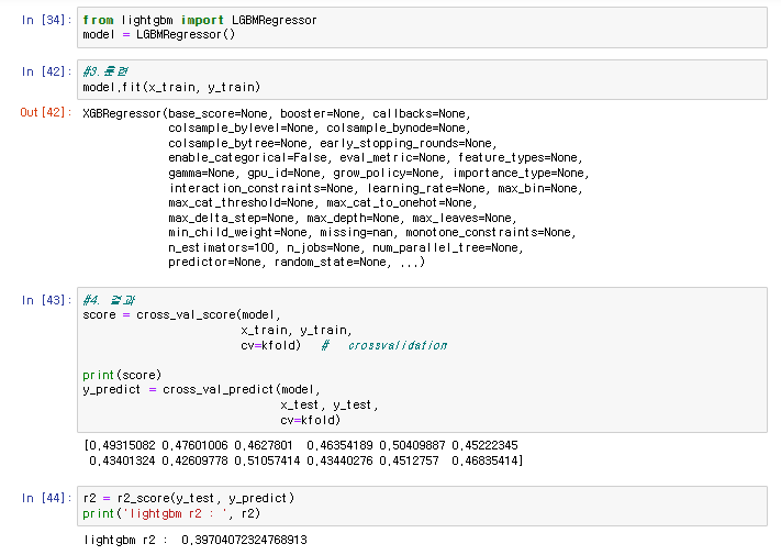
[Catboost]
pip install catboost

import numpy as np
import pandas as pd
from keras.models import Sequential
from keras.layers import Dense, Dropout
from sklearn.model_selection import train_test_split
from sklearn.metrics import r2_score

import numpy as np
from sklearn.datasets import fetch_california_housing
from sklearn.model_selection import train_test_split, KFold, StratifiedKFold
from sklearn.model_selection import cross_val_score, cross_validate, cross_val_predict
from sklearn.preprocessing import MinMaxScaler
from sklearn.utils import all_estimators
from sklearn.metrics import r2_score, accuracy_score
from sklearn.ensemble import RandomForestRegressor, RandomForestClassifier


import warnings
warnings.filterwarnings('ignore')

#1. 데이터
path = './'
datasets = pd.read_csv(path + 'train.csv')

print(datasets.columns)
#print(datasets.head(7))

# 1. x,y Data
x = datasets[['6~7_ride', '7~8_ride', '8~9_ride',
       '9~10_ride', '10~11_ride', '11~12_ride', '6~7_takeoff', '7~8_takeoff',
       '8~9_takeoff', '9~10_takeoff', '10~11_takeoff', '11~12_takeoff']]
y = datasets[['18~20_ride']]

x = x.astype('int64')

print(x.info())

x_train, x_test, y_train, y_test = train_test_split(
    x, y, train_size=0.8, shuffle=True, random_state=42 # valdiation data포함
)

#kfold
n_splits = 5
random_state=77
kfold = KFold(n_splits=n_splits,
                             shuffle=True,
                             random_state=random_state)

scaler = MinMaxScaler()
scaler.fit(x_train)
x = scaler.transform(x)
x_train = scaler.fit_transform(x_train)
x_test = scaler.transform(x_test)

from catboost import CatBoostRegressor
model = CatBoostRegressor()

#3.훈련
model.fit(x_train, y_train)

#4. 결과
score = cross_val_score(model,
                        x_train, y_train,
                        cv=kfold)   #   crossvalidation

print(score)
y_predict = cross_val_predict(model,
                              x_test, y_test,
                              cv=kfold)

r2 = r2_score(y_test, y_predict)
print('r2 : ', r2)

import matplotlib.pyplot as plt

n_features = x.shape[1]  # Use the number of features in your data
plt.barh(range(n_features), model.feature_importances_, align='center')
plt.yticks(np.arange(n_features), x.feature_names)  # Use the feature names from the Boston dataset
plt.xlabel('Feature Importance')
plt.ylabel('Features')
plt.show()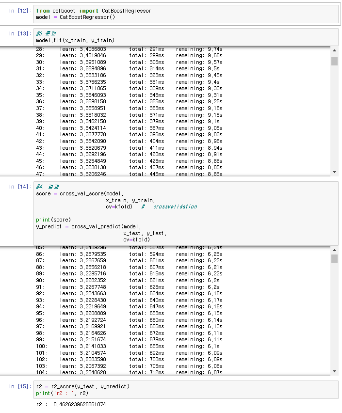
[XGboost]
pip install xgboost

pip install catboost

pip install lightgbm

import numpy as np
import pandas as pd
from keras.models import Sequential
from keras.layers import Dense, Dropout
from sklearn.model_selection import train_test_split
from sklearn.metrics import r2_score

import numpy as np
from sklearn.datasets import fetch_california_housing
from sklearn.model_selection import train_test_split, KFold, StratifiedKFold
from sklearn.model_selection import cross_val_score, cross_validate, cross_val_predict
from sklearn.preprocessing import MinMaxScaler
from sklearn.utils import all_estimators
from sklearn.metrics import r2_score, accuracy_score
from sklearn.ensemble import RandomForestRegressor, RandomForestClassifier


import warnings
warnings.filterwarnings('ignore')

#1. 데이터
path = './'
datasets = pd.read_csv(path + 'train.csv')

print(datasets.columns)
#print(datasets.head(7))

# 1. x,y Data
x = datasets[['6~7_ride', '7~8_ride', '8~9_ride',
       '9~10_ride', '10~11_ride', '11~12_ride', '6~7_takeoff', '7~8_takeoff',
       '8~9_takeoff', '9~10_takeoff', '10~11_takeoff', '11~12_takeoff']]
y = datasets[['18~20_ride']]

x = x.astype('int64')

print(x.info())

x_train, x_test, y_train, y_test = train_test_split(
    x, y, train_size=0.8, shuffle=True, random_state=42 # valdiation data포함
)

#kfold
n_splits = 5
random_state=77
kfold = KFold(n_splits=n_splits,
                             shuffle=True,
                             random_state=random_state)

scaler = MinMaxScaler()
scaler.fit(x_train)
x = scaler.transform(x)
x_train = scaler.fit_transform(x_train)
x_test = scaler.transform(x_test)

#2. 모델
from xgboost import XGBRegressor
model = XGBRegressor()

#3.훈련
model.fit(x_train, y_train)

#4. 결과
score = cross_val_score(model,
                        x_train, y_train,
                        cv=kfold)   #   crossvalidation

print(score)
y_predict = cross_val_predict(model,
                              x_test, y_test,
                              cv=kfold)

r2 = r2_score(y_test, y_predict)
print('xgboost r2 : ', r2)

import matplotlib.pyplot as plt

n_features = x.shape[1]  # Use the number of features in your data
plt.barh(range(n_features), model.feature_importances_, align='center')
plt.yticks(np.arange(n_features), x.feature_names)  # Use the feature names from the Boston dataset
plt.xlabel('Feature Importance')
plt.ylabel('Features')
plt.show()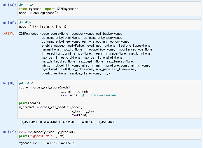
실습 2.
Feature importances 확인 및 feature 정의 후 성능 비교
반응형